How Does Stock Market Volatility Impact Returns?
Overview
The performance of three different portfolios is compared using simulated returns. Since stock market prices change in different ways over time, the three portfolios are compared during three different market volatility periods: high, average, and low. In general, stock returns are worse during periods of high volatility and better during periods of low volatility. Of course, this is not investment advice!
The portfolios are composed of SPY and TLT which are ETFs representing the S&P 500 Index and 20+ Year Treasury Bonds.
| Portfolio | Percent SPY | Percent TLT |
|---|---|---|
| Growth | 80% | 20% |
| Balanced | 65% | 35% |
| Conservative | 40% | 60% |
R programming code snippets are embedded throughout this article. The full R source code and the dataset are available on GitHub.
ETL
The source data is composed of daily returns by symbol. Dates are not aligned in the data and will be aligned in the code.
Data Validation
The loaded daily returns are compared to known year-end figures.
We will verify
- Missing data is not significant.
- Daily returns are correct.
- The annual return calculation is correct.
Check for Missing Data
start_date <- '2004-11-01'
stop_date  <- '2016-12-31'

market_data[Date >= start_date & Date <= stop_date & is.na(TLT_Return_Pct),]
market_data[Date >= start_date & Date <= stop_date & is.na(SPY_Return_Pct),]
market_data[Date >= start_date & Date <= stop_date & is.na(USGG1M_Return_Pct),]
Results
- TLT: No missing data.
- SPY: No missing data.
- USGG1M (Risk Free Rate): Missing value on ‘2015-05-08’.
Verify Returns
start_date      <- '2015-01-01'
stop_date       <- '2015-12-31'
market_data_cut <- market_data[Date >= start_date & Date <= stop_date, ]

market_data_cut$SPY_Return_Index <- (market_data_cut$SPY_Return_Pct / 100) + 1
spy_annual_return                <- (prod(market_data_cut$SPY_Return_Index,
                                          na.rm=FALSE) - 1)*100
spy_annual_return
## [1] 1.252234
market_data_cut$TLT_Return_Index  <- (market_data_cut$TLT_Return_Pct / 100) + 1
tlt_annual_return                 <- ( prod(market_data_cut$TLT_Return_Index,
                                            na.rm=FALSE) - 1)*100
tlt_annual_return
## [1] -1.787336
Results
Success. The calculated annual returns from the 2015 daily values match the expected annual returns observed in 2015.
2015 SPY return: 1.25% (source)
2015 TLT return: -1.79% (source)
Define Time Periods
Create time periods for average, high, and low, volatility periods.
Average Volatility Period
The average time period includes daily returns from every day over the 10 year period from 04/01/2007 to 03/31/2017.
## [1] 2518
⇒ There are 2,518 days in the average volatility time period.
High Volatility Period
The high volatility time period includes days where the CBOE Volatility Index “VIX” is greater than 30. Days in this time period range from 9/15/08 to 5/18/09. This time period coincides with the financial crisis.
## [1] 170
⇒ There are 170 days in the high volatility time period.
Low Volatility Period
The low volatility time period includes days where the VIX is always less than 20 and often less than 15. This time period includes dates from 11/01/04 to 1/1/07 AND from 1/4/2013 to 10/3/14.
## [1] 987
⇒ There are 987 days in the low volatility time period.
Simulation I: Normally Distributed Returns
SPY returns are simulated from a normal distribution fitted with the observed mean and standard deviation from the sample data.
SPY_mean         <- mean(SPY_daily_returns)
SPY_sd           <- sd(SPY_daily_returns)
SPY_sim_returns  <- rnorm(avg_vol_day_count,SPY_mean,SPY_sd)
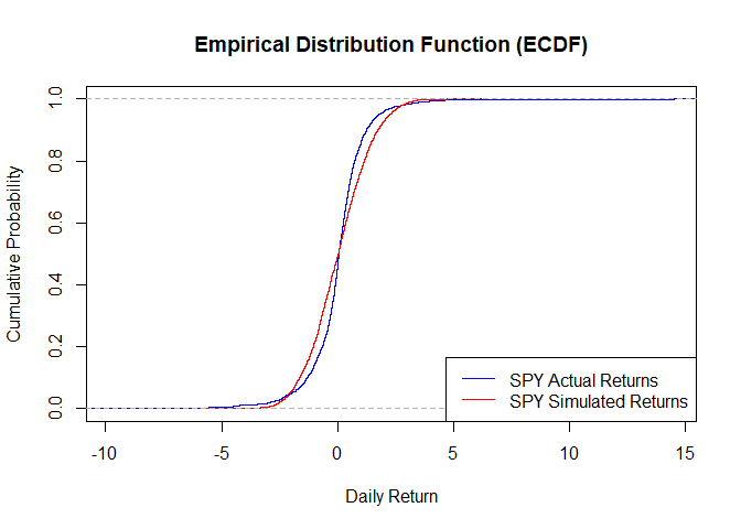
Do the simulated returns and observed returns come from the same distribution?
Two-Sample Kolmogorov-Smirnov Test
\(H_0: \)
The two samples come from a common distribution.
\(H_a: \)
The two samples do not come from a common distribution.
Test Statistic:
\(D = 0.11676\)
P-Value < .0001
Decision: Reject
\(H_0\)
.
ks.test(SPY_daily_returns, SPY_sim_returns)
    ## Warning in ks.test(SPY_daily_returns, SPY_sim_returns): p-value will be
    ## approximate in the presence of ties

    ##
    ##  Two-sample Kolmogorov-Smirnov test
    ##
    ## data:  SPY_daily_returns and SPY_sim_returns
    ## D = 0.10445, p-value = 2.35e-12
    ## alternative hypothesis: two-sided
No, the observed returns are not normally distributed.
There is significant evidence (p-value < .0001) that the simulated SPY returns are not from the same distribution as the observed SPY returns. In other words, the observed returns are not normally distributed. The normal distribution is a poor source for simulating stock returns.
Simulation II: Bootstrap Method
Stock returns are simulated by sampling dates (e.g. 2010-10-10) with replacement from the respective volatility time periods: average, high, and low volatility.
After the dates are selected, the known market data from those days are merged. One loop of the simulation generates 10 years of daily returns.
The simulation also calculates the Sharpe ratio for each return period. The Sharpe ratio represents a measure of the portfolio’s risk-adjusted return. Returns with more variability are penalized.
$$Sharpe = \frac{E|R_p - R_{rf}|}{\sqrt{var(R_p-R_{rf})}}$$where
\(R_p: \)
Daily return of the portfolio
\(R_{rf}: \)
Daily risk free rate
In other words:
Excess Return = Daily Return - Risk Free Rate
Sharpe ratio = Average(Excess Return) / sd(Excess Return)
Bootstrap Parameters
loops <- 2500                          # Number of simulations loops
days  <- avg_vol_day_count             # Days in 10 year time period
Bootstrap Function
ret.fun = function(x){
  # Generate sample dates, 'days' trading days per loop
  one_sample <- data.table(Date=sample(x, days, replace=T), key="Date")

  # Join in market data
  result <- merge(one_sample,market_data,all.x = TRUE)

  # Calculate return index
  result$growth_Return_Index        <- (result$growth_return       / 100) + 1
  result$balanced_Return_Index      <- (result$balanced_return     / 100) + 1
  result$conservative_Return_Index  <- (result$conservative_return / 100) + 1

  # Calculate annualized return
  annual_return_growth       <- (prod(result$growth_Return_Index,
                                      na.rm = FALSE) - 1)*100
  annual_return_balanced     <- (prod(result$balanced_Return_Index,
                                      na.rm = FALSE) - 1)*100
  annual_return_conservative <- (prod(result$conservative_Return_Index,
                                      na.rm = FALSE) - 1)*100

  sharpe_ratio_growth       <- mean(result$growth_excess_return)   /
                                   sd(result$growth_excess_return)
  sharpe_ratio_balanced     <- mean(result$balanced_excess_return) /
                                   sd(result$balanced_excess_return)
  sharpe_ratio_conservative <- mean(result$conservative_return)    /
                                   sd(result$conservative_excess_return)

  return(Map(cbind, annual_return_growth, annual_return_balanced,
             annual_return_conservative, sharpe_ratio_growth,
             sharpe_ratio_balanced, sharpe_ratio_conservative))
}
Average Volatility Simulation
avg_sim <- replicate(loops, ret.fun(avg_vol_days), simplify = "array")
High Volatility Simulation
hi_sim <- replicate(loops, ret.fun(high_vol_days), simplify = "array")
Low Volatility Simulation
low_sim <- replicate(loops, ret.fun(low_vol_days), simplify = "array")
Bootstrap Output: Annual Returns
Histograms of the 10 year returns are broken out by volatility period. The three portfolio groups are compared within each histogram. The median is marked with a dashed line.
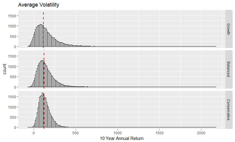
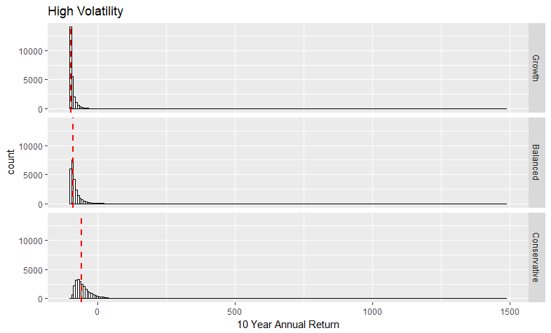
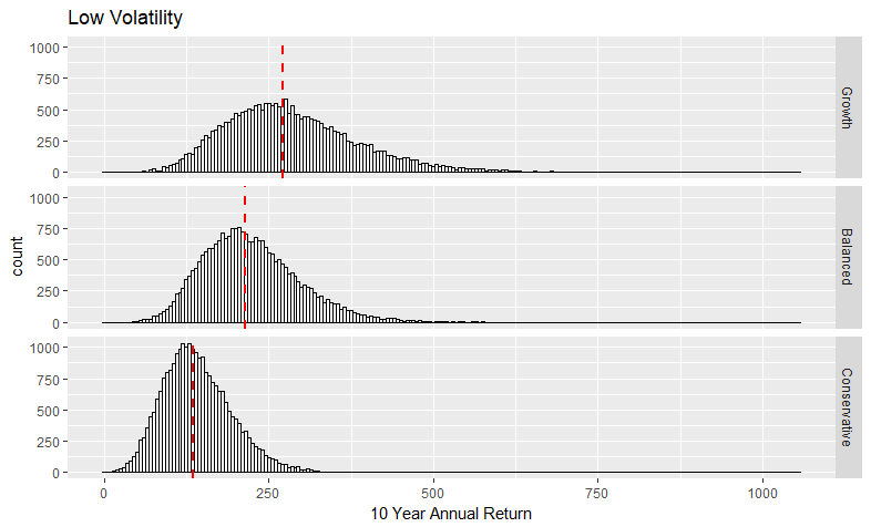
Summary statistics for the 10 year returns are grouped by volatility period and portfolio group.
pander(returns.stats)
| volatility | group | return.mean | return.median | return.sd |
|---|---|---|---|---|
| Average | Growth | 143 | 115.2 | 128 |
| Average | Balanced | 137.4 | 120.6 | 94.7 |
| Average | Conservative | 128.6 | 119 | 67.67 |
| High | Growth | -89.43 | -95.47 | 24.73 |
| High | Balanced | -81.14 | -88.75 | 26.71 |
| High | Conservative | -50.15 | -59.05 | 34.5 |
| Low | Growth | 285.2 | 272.3 | 101.4 |
| Low | Balanced | 223.2 | 215 | 73.45 |
| Low | Conservative | 141.3 | 135.7 | 52.81 |
Bootstrap Output: Sharpe Ratios
Histograms of the Sharpe ratios of the 10 year returns are broken out by volatility period. The three portfolio groups are compared within each histogram. The median is marked with a dashed line.
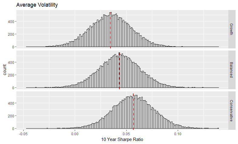
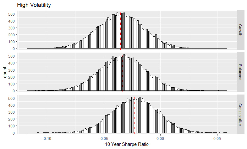
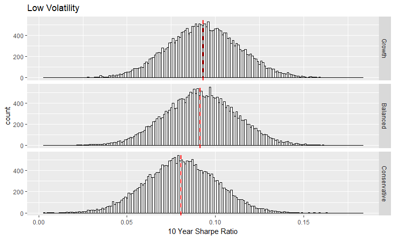
Summary statistics for the Sharpe ratios of the 10 year returns are calculated. Values are grouped by volatility period and portfolio group.
pander(sharpe.stats)
| volatility | group | sharpe.mean | sharpe.median | sharpe.sd |
|---|---|---|---|---|
| Average | Growth | 0.035 | 0.035 | 0.02 |
| Average | Balanced | 0.043 | 0.043 | 0.02 |
| Average | Conservative | 0.057 | 0.057 | 0.02 |
| High | Growth | -0.035 | -0.035 | 0.02 |
| High | Balanced | -0.033 | -0.033 | 0.02 |
| High | Conservative | -0.023 | -0.022 | 0.02 |
| Low | Growth | 0.093 | 0.093 | 0.02 |
| Low | Balanced | 0.092 | 0.091 | 0.02 |
| Low | Conservative | 0.081 | 0.08 | 0.02 |
Key Takeaways
After simulating 25,000 10-year periods, several patterns emerge. The median return referred to below is the median 10-year period return for the portfolio. Just to reiterate, this is not investment advice.
Everyone loses in extended bad markets.
In the high volatility period, all three portfolios experienced significant losses. The conservative portfolio returned a median -59%. The balanced portfolio returned a median -89% and the growth portfolio returned 7% worse than that.
The highest returns belong to the growth portfolio in the low volatility period.
All three portfolios turned in their highest median returns in the low volatility period. Median returns for the growth, balanced and conservative portfolios are 285%, 223%, and 141%, respectively.
During the average volatility period, the three portfolios have surprisingly similar returns.
Median returns are most similar during the average volatility period. Median returns for the growth, balanced and conservative portfolios are 143%, 138%, and 127%, respectively.
The conservative portfolio’s median returns are relatively similar in the low volatility period (141%) and the average volatility period (127%).
The balanced and growth portfolios perform much better in the low volatility period as compared to the average volatility period.
Unlike the conservative portfolio, the median returns for the growth and balanced portfolios get a big boost in the low volatility period. The growth median return nearly doubles to 286%. The balanced median return improves by 86% to 223%.
10-year return standard deviations are very high.
Since this simulation was run 25,000 times, the median returns should be reliable for estimating trends over the long term. However, since standard deviations are very high, any one individual 10-year period can have returns that are very different from the expected long-term value.
Sharpe ratios are relatively stable.
The Sharpe ratio is used to compare the relative riskiness of different portfolios. Specifically, it is used to detect if one portfolio is taking on extra risk in the course of achieving its returns.
Within each volatility period, there is about 1 standard deviation or less of separation between the highest and lowest median Sharpe ratios among the three portfolios. This would indicate that no individual portfolio is taking extra risk. This conclusion agrees with intuition since the portfolios are composed of diversified ETFs.
Conclusion
This experiment demonstrates that the bootstrap technique is a useful method for simulating values when an observed distribution does not conform to a common or standard distribution. In general, drawing conclusions about the financial markets is difficult due to the randomness of daily price fluctuations. However, by limiting the scope of analysis, the interaction between factors can be observed.
Acknowledgements
Thanks to Lincoln Atkinson for his helpful guide on TeX math rendering for Hugo.